Project 3: Face Morphing

By: Andi Liu

1. Introduction

In this project we will be morphing faces (my face) into someone else's face, and we will use the IMM Face Dataset to compute a mean face and extrapolate from
the mean face to create a caricature of myself. To do the morph, we will need to simultaneously warp the facial shape and cross-dissolve the image colors. We will
control the warp by using a correspondence map that is situated manually, requiring user input to align the eyes, mouth, chin, ears, etc to obtain a smooth transformation.

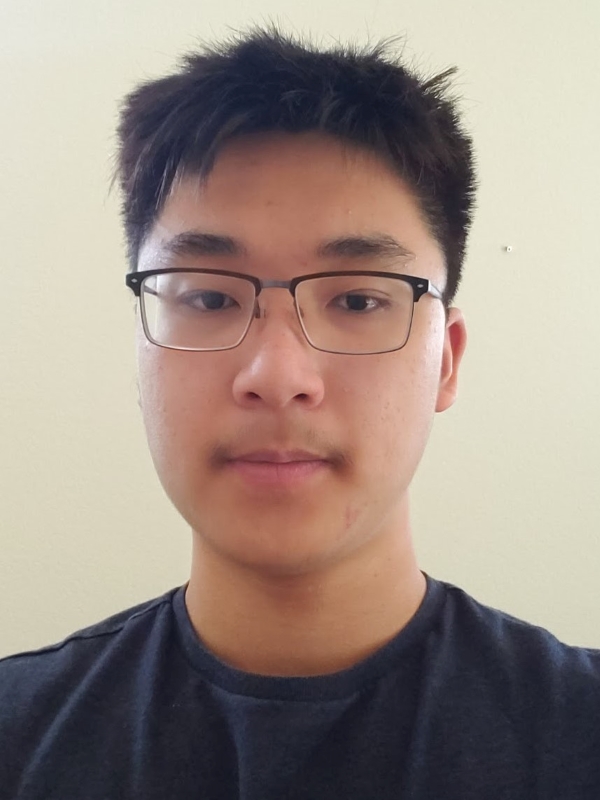
We will start with importing the image we will use throughout this project, which is my student ID image, taken over 3 years ago.

Writing the Code: Having used a variety of common functions in projects 1 and 2, I have decided to create a utils.py file for this and future projects.
This file will contain some useful functions for tasks such as importing images, displaying images, and saving images, among others.
I will add to this file throughout the semester.

2. Defining Correspondences

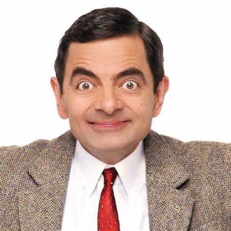
The target face we will map my face onto is that of Rowan Atkinson, acting as Mr. Bean. We import the target image as well:

The first task we need to complete for our goal is to define pairs of corresponding points on the two faces. However, to do this we need both images to be the
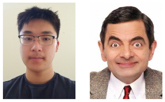
same size and shape. The image of my face is 600 by 800 pixels (the standard student ID dimensions) and the image of Mr. Bean's face is 474 by 474 pixels.
This is a mismatch that needs to be fixed. Also, for better alignment we need to crop the Mr. Bean photo to just the head and the shoulders, to better match the ID photo.
After cropping Mr. Bean to a nice round 300 by 400 pixels, we can simply downsample the ID image using sci-kit image's resize function to transform both images to
the same size and shape. The transformed images are shown below.

Now that the images are the same size and shape, we can go ahead and label the correspondences. For finding the corresponding points on both images I used the
labeling tool created by last year's student. This tool helped me click on points in both images that corresponded to one another and saved them as a json object.
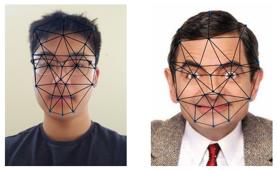
The correspondences are depicted as points in the images below. For labeling purposes, the ID image will be image 1 and the Mr Bean picture will be image 2.

Now we can create the triangulation of the correspondence points that can be used for morphing. To minimize deformation we will compute the means of the two pointsets
and pass in the mean points to scipy's Delaunay object in order to obtain a triangulation without overly skinny triangles. This triangulation is shown below:

(A bit scary looking, but that's ok.)

3. Computing the "Mid-Way Face"

Now that we have the triangulation of both images that will assist us with our morphing, we will go ahead and compute the midway face of the two images. We do this
by first finding the average of each keypoint location of the two faces, then warping both faces into that shape, and finally averaging the colors together. We will
need to implement an affine warp for each triangle into the target triangle in the mean image. This will be a function we write called computeAffine, which takes in
the vertices of two triangles and returns a matrix that maps one triangle onto the other.

Once we have our function computeAffine, we can transform each triangle in our triangulation separately, using an inverse warp of the pixels to map the original faces
to the shape of the mean face. In order to actually transform a triangle, we can use scikit-image.draw's polygon function to obtain a list of all the pixel positions in the
triangle and then apply the transform to all them using matrix multiplication to get their new positions.

Writing computeAffine: to transform one triangle into another, we need to do a translation followed by a linear transform. This means we need to use homogeneous coordinates
and a 2 by 3 transformation matrix. To actually compute the matrix, we can simply create a translation matrix and a linear transform matrix and compose them.

Note: when writing the code, I decided to use two sets of translation and linear transform matrices, a translation to move the triangle1 to the origin,
a linear transform to warp to the unit basis vectors [0,1] and [1,0], a linear transform to map to the shape of triangle2, and a final translation to the position of triangle2.
Composing these transforms gives us the final transformation matrix.

Coding problems: after a lot of debugging, I realized that the polygon function in scikit-image.draw swaps the convention for indexing order, so I had to take this into account.

Below is the process of computing the midway face, starting with the originals, then the originals warped into the shape of the midway face, and finally the midway face.

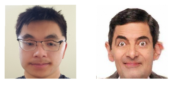
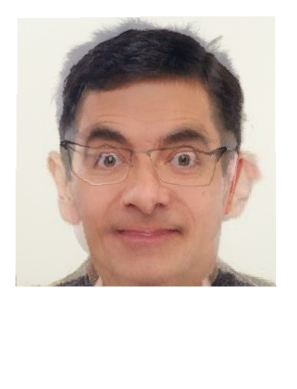
Bilinear Interpolation

In the process detailed above, the inverse mapping of the target pixels usually results in some locations that land between pixels in the original faces. In the above
process I simply set the code to take the neighboring pixel with the lowest x and y values, however this is suboptimal and results in a bit of aliasing in the warped faces.
We will now implement a version of the midway face code that uses bilinear interpolation (with scipy's griddata function) to fill in the values that fall between pixels.

Coding problems: after implementing bilinear interpolation with scipy's griddata, I immediately notice there are some missing pixels. I determine that this is because
the sci-kit image polygon function only returns pixels entirely within the polygon's interior. Below is the problematic result.

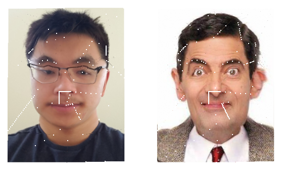
To fix this problem, I used the sci-kit image polygon_perimeter function in conjunction with the polygon function to include the perimeters of triangles. After this fix and
after making sure griddata had all the values needed for interpolation, we get the fixed bilinear interpolation result.

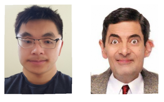
We can see that the warped faces are much better quality than the ones generated without bilinear interpolation (observe the frame of my glasses for comparison).

New Correspondences

As we can see, the correspondences defined earlier using the tool created by a student last year gives rather unsatisfactory results. I found the tool difficult to use
because the displayed position of the cursor didn't seem to match up with where the point was actually placed, and there were also issues with not being able to access the
entire image. This resulted in a significant amount of misalignment between the two images. To remedy this, I created my own simple tool for marking correspondences, that
functions within jupyter notebook. I depict the correspondences marked using my own tool below, as well as the warped faces and improved midway face generated from them.

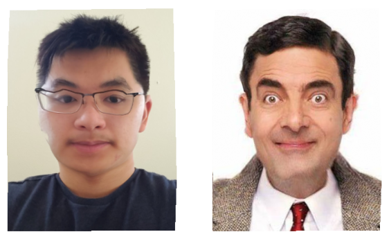
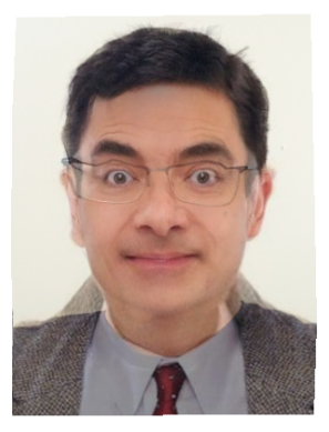
As we can see, the alignment is drastically improved with better correspondence marking. I also used more correspondence points than previously, which also improved the quality.
There are still some alignment issues around the neck area, but that is because the image of Mr. Bean has his shoulders raised much higher than in my photo. However the alignment
along the hair, ears, and face is dramatically better.

4. The Morph Sequence

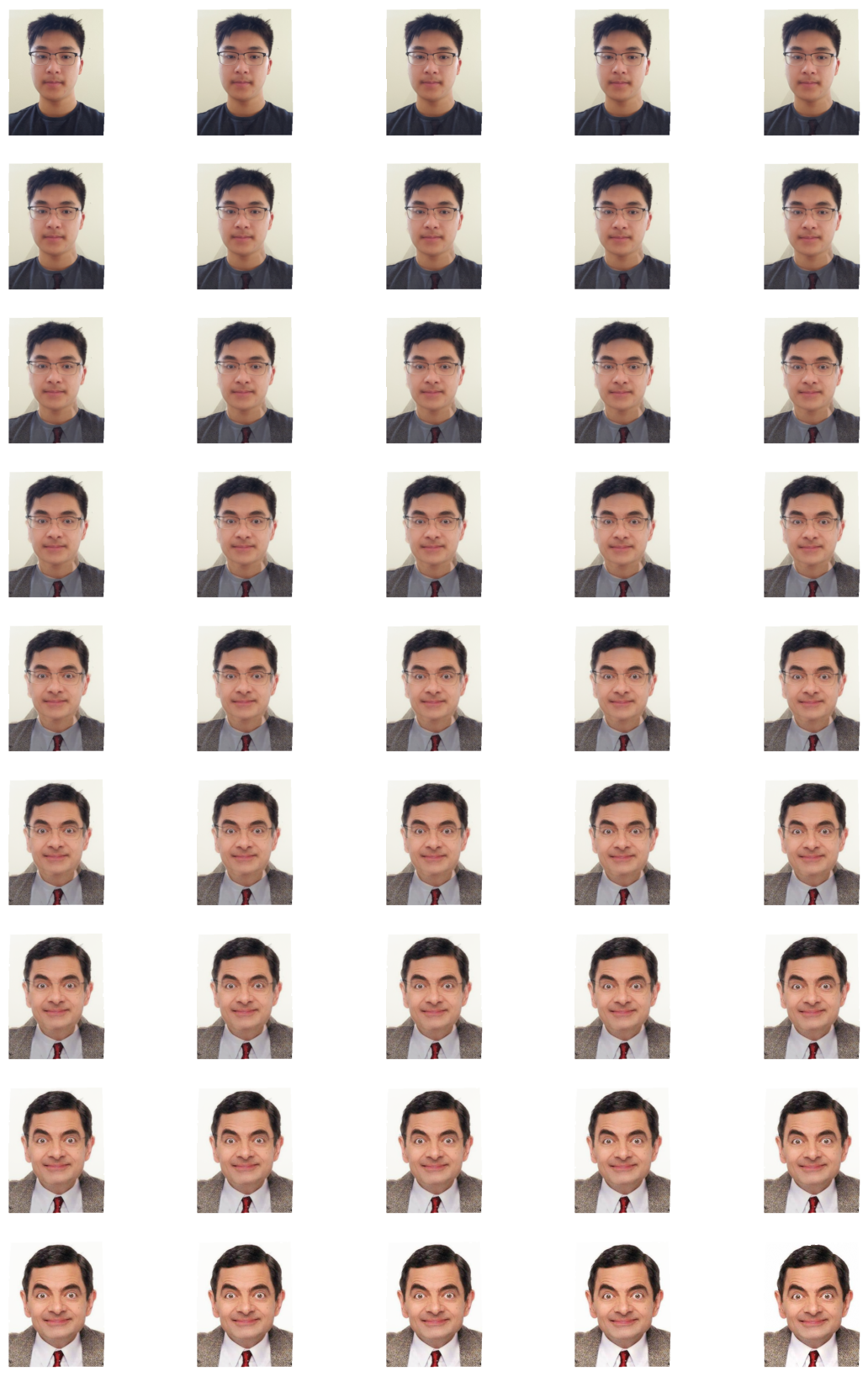
Next we will create a more general function that mixes the shape and color of the two faces to specified degrees. This function will first warp the shapes of the faces
to an intermediate shape controlled by a parameter, warp_frac, and then it will colorize this face by cross-dissolving the color to a degree controlled by another parameter,
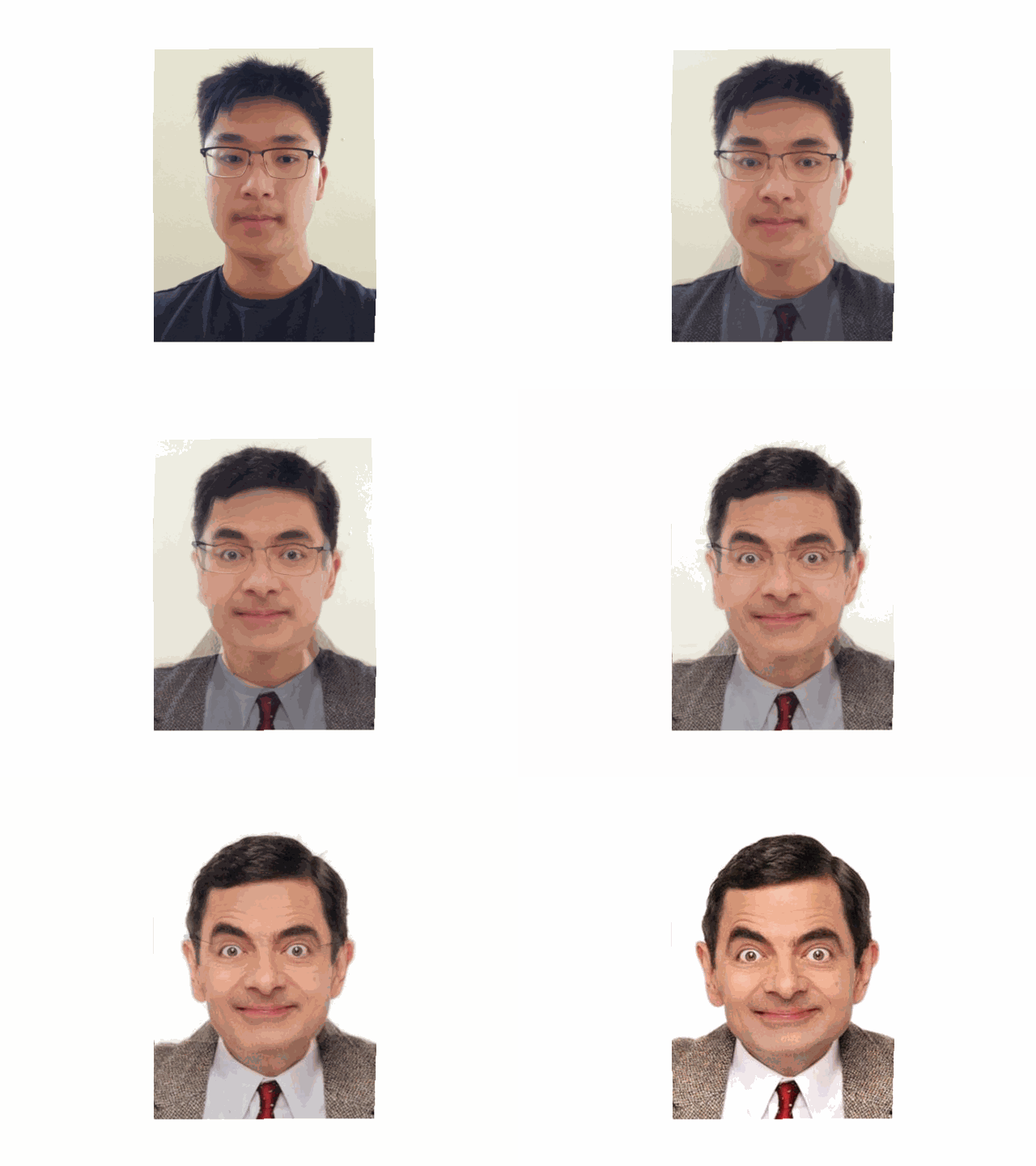
dissolve_frac. We can apply this function to create an animation morphing my face into Mr. Bean's face. For the purposes of this animation we are doing interpolation, so both
parameters will lie between 0 and 1, inclusive.

Below we can see each of the 45 frames of the animation.

Using these generated frames, we will combine them into a gif, shown below:

5. The Mean Face of a Population

For this part of the project, we will be using a 1999 dataset of faces from Caltech. (Link) The data consists of 450 annotated images of 27 unique individuals. We will use this
dataset to compute an average face shape,and morph each of the faces in the database into the mean shape. Then, we will compute the average face of the population.

To speed up processing time, I used only half of the dataset, which shouldn't affect much since there are only 27 individuals whose faces are depicted. Shown below is the
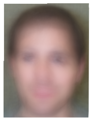
mean face computed using the correspondence points provided along with the dataset, as well as 9 example images of faces morphed to the mean shape.

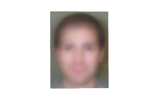
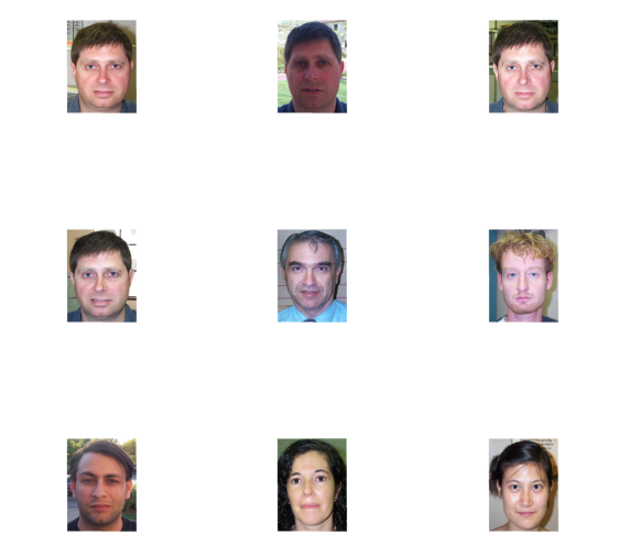
As we can see, the mean face is rather blurry, but we can still make out some general features like the eyes, nose, ears, and mouth. Additionally there is practically no warping
of the example images. This is because the dataset only came with four labelled points per image, and those points were chosen so that the faces are only roughly in the same place.
As a result the alignment we get is quite bad. However, we can still try and use this mean face to obtain a mean facial shape. We will warp my face into the mean facial shape, and the
mean face into my facial shape. Since our dataset did not come with labelling of the important facial features (eyes, ears, nose, mouth, etc) I will have to label these points manually
to do the morphing between my face and mean face.

Below is the labelled correspondence points between my face and the mean face.

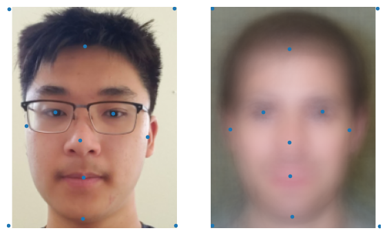
And here is my face morphed into the shape of the mean face, and the mean face morphed into the shape of my face, respectively.

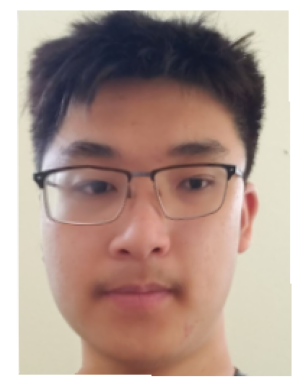
It would appear that the mean face has eyes that are vertically misaligned. Or more likely, the correspondence points are slightly misplaced. The blurriness of the mean image makes it
very difficult to properly discern where the important facial features are. We would get better results if the mean were less blurry. In order to get a less blurry mean, we need better alignment
between the faces of the dataset, which calls for more correspondence points. Once again, the lack of labelled points in our dataset is causing problems. We now have no choice but to manually
add some correspondence points to our data.

Augmenting the Data: Improving the Mean Face

The main issue with our data is that there are not enough labelled correspondence points. We will remedy this by add more manually. Furthermore, we can speed up processing times by selecting a
smaller subset of the images. Since there are only 27 individuals, we really only need 1 or 2 images of each individual in our dataset. For this particular project we don't really need the
variety of angles and illuminations provided by the full dataset. So, for each individual we will just choose 2 images with illumination and lighting closest to my own picture.

Below is the smaller dataset with the new correspondence points depicted.

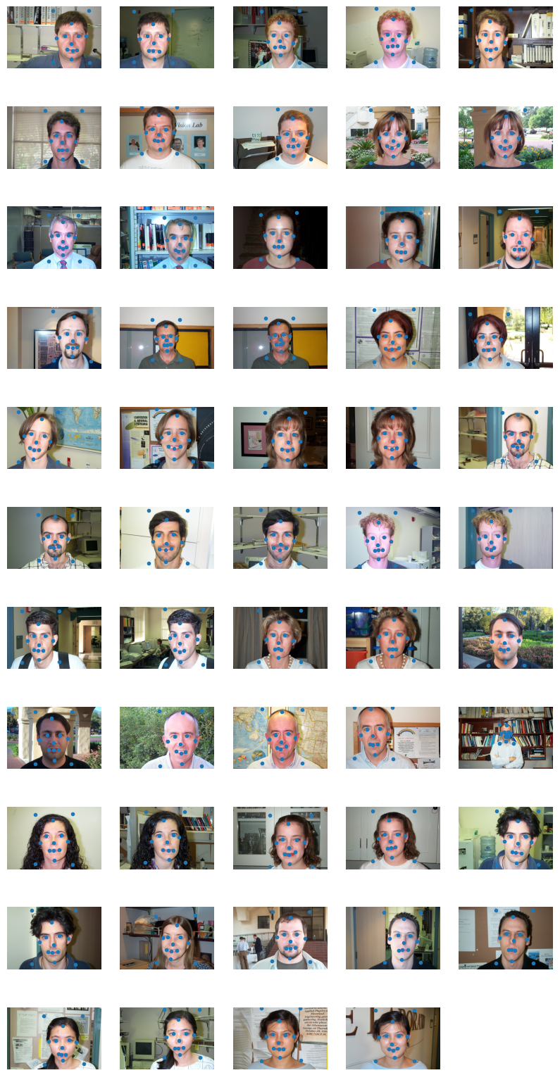
Now if we compute the mean face of this smaller dataset, we should get a better quality mean face, depicted below.

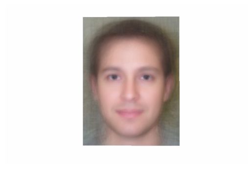
Indeed, we can see that the population mean face is much clearer when more correspondence points are added. However, the cost of this clarity in the mean is more individual morphing of
any given face, as we can see with some examples below:

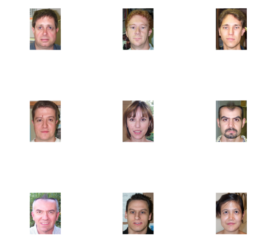
As we can see, adding the correspondence points allowed for more detailed morphing of the facial features, which creates more warping when we morph each individual face to the mean shape.

Once again, we will warp my face to the shape of the mean face, and the mean face to the shape of my face. This time we see much better results, because the mean face is much clearer., and
there is less error from placing the correspondence points.

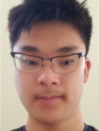
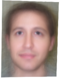
6. Caricatures: Extrapolating From the Mean

We will now try and extrapolate from the population mean we obtained in the last part, using my photo to create caricatures of myself. We will do this by using the morph function, which allows
for the warp_frac and dissolve_frac parameters to be set to values less than 0. Since 0 is my original image and 1 is the mean face, values less than 0 would be extrapolating towards the "my-face direction".

Below are some extrapolations in both the color and shape dimensions.

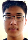
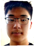
We get some pretty funny-looking caricatures when we extrapolate on shape. The extrapolations on color just seem to make the skin colors darker. Unfortunately, because the images were fairly
low-resolution to begin, the resolutions on the shape extrapolations become even worse the more we extrapolate.

Bells and Whistles: Principle Component Analysis

For the final piece of this project, we will perform a Principle Component Analysis on the Database of faces, obtaining a low-dimensional basis that we can use to create more caricatures.
In the previous section, we extrapolated using only a single direction vector, which was the difference vector between my face and the population mean. By obtaining a low-dimensional basis for
the space of facial shapes, we can obtain a greater variation of caricatures. The space of facial shapes we analyze will be defined by the 14 correspondence points in our augmented database.
For complete control over facial variations, we could include the colors of each pixel (so that our space entails both shape and color), but since our goal is to create more caricatures, a PCA
of the facial-shape space will suffice. To visualize the bases we obtain from the PCA, we will add or subtract certain amount of each basis from the mean.

Upon performing the singular value decomposition of our data, we find that only the first three basis vectors are really significant. So, we will be using a low-dimensional space with 3 dimensions
to generate our caricatures.

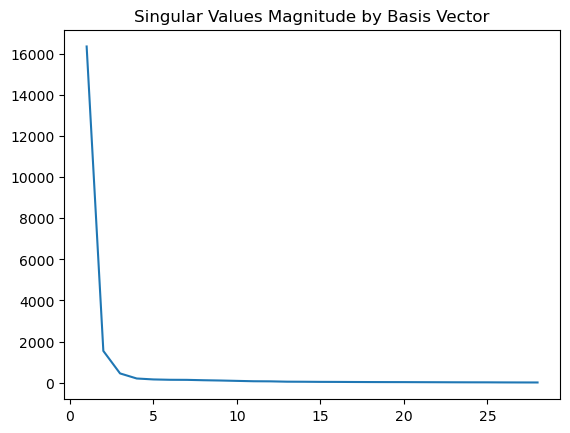
Indeed, the singular values with significant magnitudes are only the first three. Let's visualize what the corresponding basis vectors are.

Visualizing the first basis vector, we see that the size of the image changes, because the original four correspondence points that the dataset came with drew a box around each face.
Upon subsequent exploration, we notice that every basis vector includes some kind of resizing. We do not want this resizing in our basis vectors, so we will redo the PCA, but this time
removing the four corner points from our dataset.

As we can see, the first basis vector has a resizing element to it, as do the next four basis vectors. We will strip the dataset of the corner points and redo the analysis

Upon redoing the analysis, I found that the more interesting facial morphs are in fact not the most significant vectors. For instance, the vector controlling facial width is the sixth vector
and the seventh and eighth vectors control the degree of frowning vs smiling. The magnitude of the singular values does not really tell us much about the importance of the basis vector.

Below I show the effects of drastically adding or subtracting the first 10 basis vectors to/from the mean face.

First basis vector

Second basis vector

Third basis vector

Fourth basis vector

Fifth basis vector

Sixth basis vector

Seventh basis vector

Eighth basis vector

Ninth basis vector

Tenth basis vector

We can see that the PCA basis gives us much better results in the facial morphing than in the normal basis. We have relatively fine-tuned control over the facial expressions and
facial shape.

Caricatures, but Better

Now that we have very fine-tuned control over the facial shape, we can make some more caricatures of myself, in each of the PCA bases dimensions.

Below is my face warped in both directions of each of the first 10 basis vectors. (Adding and subtracting the basis vector times some multiple).

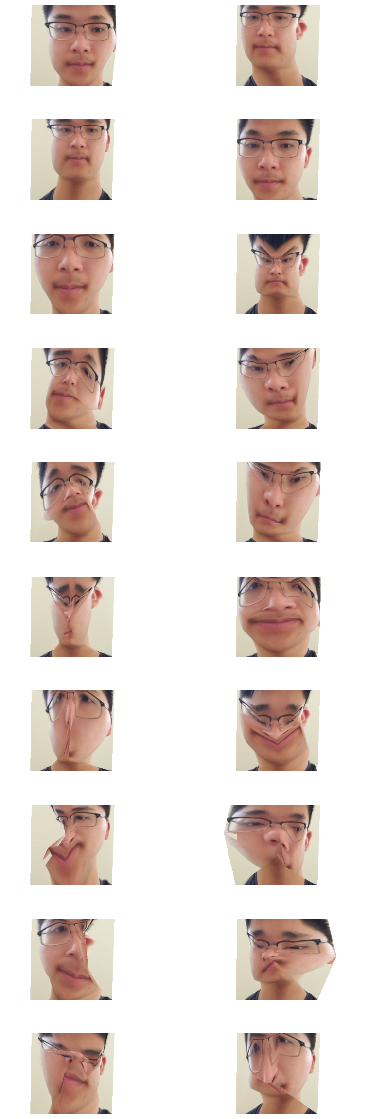
As we can see, we get much more varied caricatures, with some very interesting ones, and we can generate even more by combining the basis vector displacements.